Diagnostics: when to trust an estimate • isoniche

library(isoniche)

Isodars are estimated from the spread of a species’ densities across replicates, so a species needs enough replicates, enough individuals and a consistent habitat preference for its niche breadth to be estimated well. Many species in a typical community data set will not meet these requirements. niche_breadth() never stops on such a species: it returns an estimate where it can, and records each potential problem as a logical flag_* column. This vignette explains each flag and what to do about it.

All species of the Moorea data

nb <- niche_breadth(moorea_fish, species = "species", site = "site",
                    habitat = "habitat", abundance = "abundance",
                    n_boot = 0, seed = 1)
summary(nb)
#> Niche breadth for 325 species
#>   DD niche breadth at: asymptote; bootstrap replicates: 0
#>   with DI and DD estimates: 167
#>   without warning flags:    32
#> 
#> Estimates (quartiles):
#>                     min q25 median    q75  max
#> nb_di                 0   0  0.181  0.442    1
#> spillover_abundance   1   1  9.000 39.500 5085
#> nb_dd                 0   0  0.001  0.125    1
#> 
#> Flags raised (species):
#>   few_sites            158  fewer sites than min_sites
#>                             -> group nearby sites (group_sites()) or treat as unreliable
#>   fit_failed            98  isodars could not be fitted
#>                             -> see the 'note' column
#>   undersampled          97  zeros in a habitat sampled at too few sites to call it absent
#>                             -> sample more sites, or name absent habitats with 'absent'
#>   intercept_noise       96  isodar intercepts do not differ from sampling noise
#>                             -> no evidence that niche breadth changes with abundance; report DD niche breadth
#>   poor_fit              90  a line does not describe the data well, or the pairwise isodars disagree
#>                             -> check the isodars (fit_isodars()); try the other method
#>   low_abundance         85  small counts per site, or mostly zeros
#>                             -> group sites, or report as unreliable; estimates rest on few individuals
#>   no_di                 60  no total abundance occupies every used habitat
#>                             -> check the isodars; the least-favoured habitat may never fill
#>   di_extrapolation      37  spillover abundance outside the range of observed site totals
#>                             -> DI niche breadth is extrapolated; interpret with care
#>   dd_extrapolation      30  the data do not reach the abundances that determine DD niche breadth
#>                             -> DD niche breadth is extrapolated; interpret with care
#>   few_pair_sites         5  a pair of used habitats shares fewer than min_pair_sites sites
#>                             -> use dim = "ndim" with ndim_method = "latent", or group sites
#>   reversal             133  habitats change rank along the niche breadth curve
#>                             -> informational: compare species at a stated abundance (see iai_curve())
#>   abandoned            113  a used habitat is abandoned at high density
#>                             -> informational: the habitat counts for DI but not for DD niche breadth
#> 
#> See vignette("diagnostics") for details. Thresholds are set with niche_breadth(diagnostics = ).

In a data set of 13 sites, most rare species cannot be analysed. This is expected: the same species would also give unreliable classic niche breadth values, but without any warning.

The flags

Thresholds are arguments of niche_breadth(), set through diagnostics (e.g. diagnostics = list(min_sites = 8)); the defaults are given below.

Data

few_sites: fewer than min_sites (10) replicates with the species. Isodars from few points are imprecise. Group nearby sites (group_sites(); see vignette("data-preparation")) or treat the species as unreliable.
few_pair_sites: some pair of used habitats was sampled together at fewer than min_pair_sites (5) sites, so its pairwise isodar is poorly estimated. Use the n-dimensional isodar with ndim_method = "latent", or group sites.
low_abundance: the median site total is below min_median_count (5) individuals, or more than max_zero_share (half) of the counts in used habitats are zeros. Densities are then dominated by sampling noise.
undersampled: a habitat without records was sampled at too few sites to call it absent. Sample more sites, or decide on ecological grounds and name absent habitats with absent.

Fit

fit_failed: the isodars could not be fitted; the reason is in the note column. Most often the species has too few sites.
disconnected: some habitats never occur together at a site, so their relationship cannot be estimated.
poor_fit: for the n-dimensional isodar, the line explains less than min_var_explained (50%) of the variance; for pairwise isodars, the isodars of three habitats contradict each other (the product of two slopes differs from the third by more than a factor max_slope_ratio, 2, or in sign). Habitat selection may not follow a single isodar, or the data are too noisy. Look at the isodars with fit_isodars(), and try the other method (dim = "ndim" or "pairwise").
no_di: no total abundance up to max_search puts an individual in every used habitat: the least-favoured habitat is predicted never to fill.
intercept_noise: the isodar intercepts do not differ from those expected by sampling alone (see below). The data then give no evidence that niche breadth changes with abundance: with zero intercepts, the isodars pass through the origin and DI and DD niche breadth are equal. Report a single value, DD niche breadth, which rests on the slopes only and is the better estimated. With few sites the test has little power, so this flag does not show that the intercepts are zero.

Extrapolation

di_extrapolation: the spillover abundance lies outside the observed range of site totals by more than a factor extrapolation_ratio (2).
dd_extrapolation: the largest site total is below twice the spillover abundance, so the data never reach the halfway point of the curve towards DD niche breadth.

Both are extrapolations of the fitted isodars; the estimates may be right, but rest on the assumption that the isodars hold beyond the data.

Uncertainty

unstable_bootstrap (only with n_boot > 0): more than max_failed_share (10%) of bootstrap replicates failed, or a confidence interval is wider than max_ci_width (0.5). Increase n_boot; if the interval stays wide, the data cannot resolve the species’ niche breadth.

Informational

reversal: two habitats swap rank as abundance increases; the abundances are in the reversals column. Niche breadth can then change non-monotonically with abundance, so compare species at a stated abundance.
abandoned: a habitat used at low abundance is predicted to be empty at high abundance; it counts for DI but not DD niche breadth.

Is the intercept more than noise?

When a species is rare, counts in its habitats are small and their ratios noisy, which alone produces isodar intercepts. niche_breadth() tests whether the observed intercepts exceed this: it simulates n_null (199) data sets in which each site’s individuals are redistributed among its habitats at random, in proportion to the species’ overall density in each habitat (no density dependence), refits the isodars, and compares the observed intercepts with the simulated ones. intercept_p is the smallest Holm-corrected p-value; the species is flagged when it exceeds alpha (0.05). The test needs integer counts.

noisy <- nb[nb$flag_intercept_noise & !nb$flag_few_sites, ]
noisy[c("species", "nb_di", "nb_dd", "intercept_p")]
#> # A tibble: 64 × 4
#>    species                       nb_di   nb_dd intercept_p
#>    <chr>                         <dbl>   <dbl>       <dbl>
#>  1 Acanthurus lineatus        NA       0.0675        1    
#>  2 Acanthurus nigroris        NA       0.00533       0.24 
#>  3 Acanthurus olivaceus       NA       0.00127       0.15 
#>  4 Anampses caeruleopunctatus  0.0537  0.0537        0.746
#>  5 Anampses melanurus          0.0519  0.0379        0.49 
#>  6 Arothron meleagris          0.243   0.209         0.155
#>  7 Cantherhines dumerilii     NA       0             0.172
#>  8 Cantherhines pardalis       0.00157 0.00152       0.887
#>  9 Canthigaster bennetti       0.213   0.126         0.06 
#> 10 Caracanthus maculatus       0.288   0             0.15 
#> # ℹ 54 more rows
#> Abundances are per site (equal effort in every site and habitat).

Looking at a flagged species

Diagnostics are a starting point. For a flagged species, look at its isodars and curve:

sp <- "Acanthurus nigrofuscus"
nb[nb$species == sp, c("nb_di", "nb_dd", "var_explained", "flags")]
#> # A tibble: 1 × 4
#>   nb_di nb_dd var_explained flags             
#>   <dbl> <dbl>         <dbl> <chr>             
#> 1 0.468 0.365            NA reversal, poor_fit
#> Abundances are per site (equal effort in every site and habitat).
fit <- fit_isodars(moorea_fish[moorea_fish$species == sp, ], site = "site",
                   habitat = "habitat", abundance = "abundance")
fit$fit[[1]]
#> # A tibble: 3 × 7
#>   habitat_x    habitat_y     intercept  slope    sd n_sites flipped
#>   <chr>        <chr>             <dbl>  <dbl> <dbl>   <int> <lgl>  
#> 1 barrier_reef fringing_reef     0.553 0.916   59.3      13 FALSE  
#> 2 outer_slope  barrier_reef     49.6   0.265   66.9      13 TRUE   
#> 3 outer_slope  fringing_reef    86.6   0.0755  70.9      13 TRUE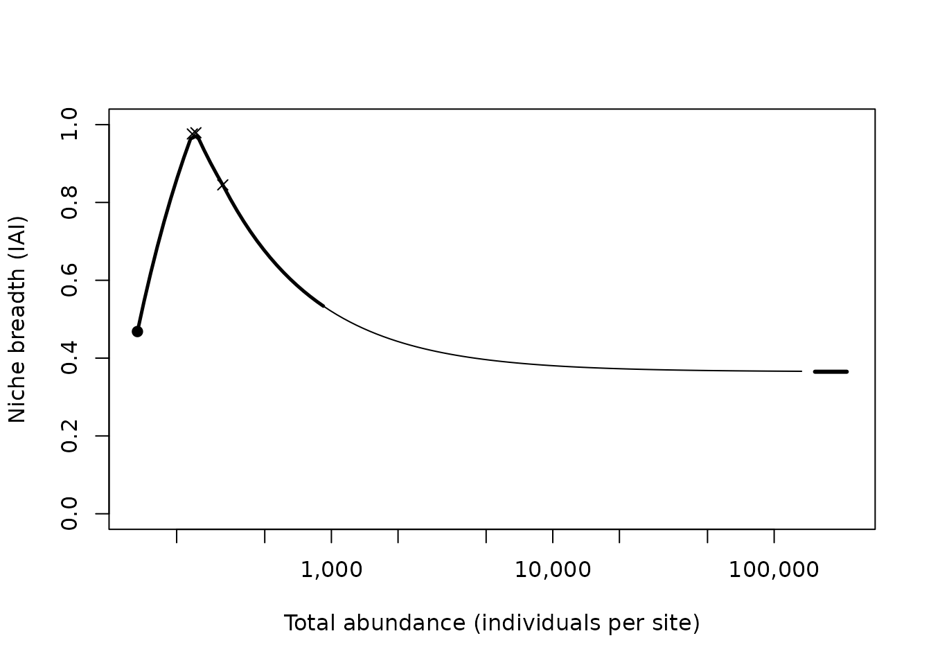

plot(iai_curve(fit))

nb$reversals[[which(nb$species == sp)]]
#>   total_abundance     habitat_1    habitat_2 niche_breadth
#> 2        235.4562  barrier_reef  outer_slope     0.9759597
#> 3        244.3702 fringing_reef  outer_slope     0.9791916
#> 1        323.1334 fringing_reef barrier_reef     0.8452180

When rare, this species lives on the fringing and barrier reefs: both isodars against the outer slope have large intercepts. But the outer slope fills fastest as abundance rises (the reefs gain only 0.27 and 0.08 individuals per individual on the outer slope), so it overtakes both reefs at a few hundred individuals, the ranking of habitats changes and niche breadth first rises, then falls. Here the pairwise isodars are also somewhat inconsistent with each other (poor_fit). Neither DI nor DD niche breadth alone describes such a species well; the curve does.

A workflow

Run check_coverage() and drop species or habitats that are clearly undersampled.
Run niche_breadth() with n_boot = 0 on all species; look at summary().
Decide how to handle each warning flag (for example: drop species with fit_failed, few_sites or low_abundance; report DI and DD niche breadth separately only where intercept_noise is not raised).
Rerun on the retained species with n_boot = 999 or more, and check unstable_bootstrap.
Report the thresholds and how many species each rule removed.